Probability distributions

In probability theory and statistics, a probability distribution is the mathematical function that gives the probabilities of occurrence of different possible outcomes for an experiment. It is a mathematical description of a random phenomenon in terms of its sample space and the probabilities of events (subsets of the sample space).

Introduction

Probability is the science of uncertainty. It provides precise mathematical rules for understanding and analyzing our own ignorance. It does not tell us tomorrow’s weather or next week’s stock prices; rather, it gives us a framework for working with our limited knowledge and for making sensible decisions based on what we do and do not know. (citee)

Terminology

Sample space

In probability theory, the sample space refers to the set of all possible outcomes of a random experiment. It is denoted by the symbol Ω (capital omega).

• Let's consider an example of rolling a fair six-sided die. The sample space in this case would be {1, 2, 3, 4, 5, 6}, as these are the possible outcomes of the experiment. Each number represents the face of the die that may appear when it is rolled.

Random variable

Random variable takes values from a sample space. In contrast, probabilities describe which values and set of values are more likely to be taken out of the sample space. Random variable must be quantified, therefore, it assigns a numerical value to each possible outcome in the sample space.

• For example, if the sample space for flipping a coin is {heads, tails}, then we can assign a random variable Y such that Y = 1 when heads land and Y = 0 when tails land. However, we can assign any number for these variables. 0 and 1 are just more convenient.

• Because random variables are defined to be functions of the outcome s, and because the outcome s is assumed to be random (i.e., to take on different values with different probabilities), it follows that the value of a random variable will itself be random (as the name implies).

Specifically, if X is a random variable, then what is the probability that X will equal some particular value x? Well, X = x precisely when the outcome s is chosen such that X(s) = x.

• Exercise
  • Suppose that a coin is tossed twice so that the sample space is S = {HH, HT, TH, TT}. Let X represent the number of heads that can come up. With each sample point we can associate a number for X as shown in Table 1. Thus, for example, in the case of HH (i.e., 2 heads), X = 2 while for TH (1 head), X 􏰂= 1. It follows that X is a random variable.

PMF vs. PDF vs. CDF

In probability theory there are 3 functions that might be little confusing for some people. Let's make the differences clear.

Probability mass function (PMF)

• The probability mass function, denoted as P(X = x), is used for discrete random variables. It assigns probabilities to each possible value that the random variable can take. The PMF gives the probability that the random variable equals a specific value.

Cumulative distribution function (CDF)

• The cumulative distribution function, denoted as F(x), describes the probability that a random variable takes on a value less than or equal to a given value x. It gives the cumulative probability up to a specific point.
• Since the PDF is the derivative of the CDF, the CDF can be obtained from PDF by integration

Probability density function (PDF)

To determine the distribution of a discrete random variable we can either provide its PMF or CDF. For continuous random variables, the CDF is well-defined so we can provide the CDF. However, the PMF does not work for continuous random variables, because for a continuous random variable P(X=x)=0 for all x ∈ ℝ. Instead, we can usually define the probability density function (PDF). The PDF is the density of probability rather than the probability mass. The concept is very similar to mass density in physics: its unit is probability per unit length.

• The probability density function (PDF) is a function used to describe the probability distribution of a continuous random variable. Unlike discrete random variables, which have a countable set of possible values, continuous random variables can take on any value within a specified range.

• The PDF, denoted as f(x), represents the density of the probability distribution of a continuous random variable at a given point x. It provides information about the likelihood of the random variable taking on a specific value or falling within a specific range of values.
• Since the PDF is the derivative of the CDF, the CDF can be obtained from PDF by integration

Distribution Functions for Random Variables

The distribution function provides important information about the probabilities associated with different values of a random variable. It can be used to calculate probabilities for specific events or to obtain other statistical properties of the random variable.

• It gives the probability that the random variable takes on a value less than or equal to a given value.

The distribution function of a random variable X, denoted as F(x), is defined as:

• F(x) = P(X ≤ x)

where x is any real number, and P(X ≤ x) is the probability that the random variable X is less than or equal to x.

Distribution Functions for Discrete Random Variables

If X takes on only a finite number of values x1, x2, . . . , xn, then the distribution function is given by

Discrete uniform distribution

Example

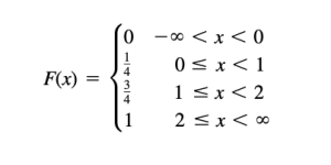
The following function:

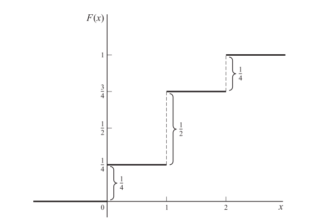
Can be graphed as follows:

1. The magnitudes of the jumps are 1/4, 1/2, 1/4 which are precisely the probabilities from the function. This fact enables one to obtain the probability function from the distribution function.
2. Because of the appearance of the graph it is often called a staircase function or step function.
3. The value of the function at an integer is obtained from the higher step; thus the value at 1 is 4 and not 4. This is expressed mathematically by stating that the distribution function is continuous from the right at 0, 1, 2. 3. As we proceed from left to right (i.e. going upstairs), the distribution function either remains the same or

increases, taking on values from 0 to 1. Because of this, it is said to be a monotonically increasing function.

Distribution Functions for Continuous Variables

A nondiscrete random variable X is said to be absolutely continuous, or simply continuous, if its distribution function may be represented as

where the function f(x) has the properties

Special Probability Distributions

The Binomial Distributions

• Suppose that we have an experiment such as tossing a coin repeatedly or choosing a marble from an urn repeatedly.
• Each toss or selection is called a trial.
• In any single trial there will be a probability associated with a particular event such as head on the coin, 4 on the die, or selection of a red marble. In some cases this probability will not change from one trial to the next (as in tossing a coin or die).
• Such trials are then said to be independent and are often called Bernoulli trials after James Bernoulli who investigated them at the end of the seventeenth century.

Let p be the probability that an event will happen in any single Bernoulli trial (called the probability of success). Then q 􏰂 1 􏰁 p is the probability that the event will fail to happen in any single trial (called the probability of failure). The probability that the event will happen exactly x times in n trials (i.e., successes and n 􏰁 x failures will occur) is given by the probability function

The key characteristics of a binomial distribution are as follows:

1. The trials are independent: The outcome of each trial does not depend on the outcome of any other trial.
2. Each trial has two possible outcomes: success or failure.
3. The probability of success remains constant across all trials, denoted as p.
4. The number of trials is fixed, denoted as n.

Example

The probability of getting exactly 2 heads in 6 tosses of a fair coin is:

The Normal Distributions