Difference between revisions of "Monte Carlo method in simulations"
(→Examples of Monte Carlo Simulations for Students) |
(→Markov-Chain-Monte-Carlo Simulation) |
||
| (12 intermediate revisions by the same user not shown) | |||
| Line 2: | Line 2: | ||
== Introduction == | == Introduction == | ||
| − | Monte Carlo simulation is a mathematical technique used to simulate the possible outcomes of an uncertain event. Instead of fixed inputs, a probability distribution is used as a parameter at at least one point. By generating random probabilities as an input, a set of different outcomes and the probability of this outcomes can be generated through repeated simulation. | + | Monte Carlo simulation is a mathematical technique used to simulate the possible outcomes of an uncertain event. Instead of fixed inputs, a probability distribution is used as a parameter at at least one point. By generating random probabilities as an input, a set of different outcomes and the probability of this outcomes can be generated through repeated simulation. [[Pseudorandom number generators]] by computers plays an important role in this. <ref name="IBM"> IBM Cloud Education. What is Monte Carlo Simulation?[2020-01-24]. Available at: https://www.ibm.com/cloud/learn/monte-carlo-simulation#toc-what-is-mo-b7t4vgvP</ref> |
The first well-known experiment that used randomness to solve a problem was "Buffon's Needle". <ref name="Harrison">Harrison, Robert L. Introduction To Monte Carlo Simulation. AIP Conf Proc. 2010 January 5; 1204: 17–21. doi:10.1063/1.3295638</ref> The French scientist Georges Louis LeClerc, Comte de Buffon asked in the 18th century the question with what probability a randomly thrown needle intersects a grid of parallel lines. Only a few years later he was able to prove that this probability is 2L/Dπ (D > L). Let L be the length of the needle and D the distance between the lines. <ref name="Richeson">Richeson, David. A π-less Buffon's Needle Problem. Mathematics Magazine , Dec., 2006, Vol. 79, No. 5 (Dec., 2006), pp. 385-389. Available at: hhttps://www.jstor.org/stable/27642977</ref> In his first experiments, LeClerc allegedly threw baguettes over his shoulder onto a tiled floor.<ref name="Harrison">Harrison, Robert L. Introduction To Monte Carlo Simulation. AIP Conf Proc. 2010 January 5; 1204: 17–21. doi:10.1063/1.3295638</ref> In 1812, the French scientist Pierre-Simon Laplace suggested that this experiment could be used to determine the number π.<ref name="Harrison">Harrison, Robert L. Introduction To Monte Carlo Simulation. AIP Conf Proc. 2010 January 5; 1204: 17–21. doi:10.1063/1.3295638</ref> In 1901, the scientist Mario Lazzarini was able to determine the number π to 6 decimal places by throwing needles on a grid of parallel lines, and that after only 3408 throws.<ref name="Harrison">Harrison, Robert L. Introduction To Monte Carlo Simulation. AIP Conf Proc. 2010 January 5; 1204: 17–21. doi:10.1063/1.3295638</ref> However, this result is also doubted by scientists or also described as a stroke of luck. This is because in order to determine the number π to 6 decimal places in a 95% confidence interval, one would theoretically have to throw at least 134 trillion needles.<ref name="Badger">Badger, Lee. Lazzarini's Lucky Approximation of π. Mathematics Magazine , Apr., 1994, Vol. 67, No. 2 (Apr., 1994), pp. 83-91. Available at: https://www.jstor.org/stable/2690682</ref> Nowadays, these experiments can be simulated much faster and more efficiently with the help of computers. One possible way is included in the examples. | The first well-known experiment that used randomness to solve a problem was "Buffon's Needle". <ref name="Harrison">Harrison, Robert L. Introduction To Monte Carlo Simulation. AIP Conf Proc. 2010 January 5; 1204: 17–21. doi:10.1063/1.3295638</ref> The French scientist Georges Louis LeClerc, Comte de Buffon asked in the 18th century the question with what probability a randomly thrown needle intersects a grid of parallel lines. Only a few years later he was able to prove that this probability is 2L/Dπ (D > L). Let L be the length of the needle and D the distance between the lines. <ref name="Richeson">Richeson, David. A π-less Buffon's Needle Problem. Mathematics Magazine , Dec., 2006, Vol. 79, No. 5 (Dec., 2006), pp. 385-389. Available at: hhttps://www.jstor.org/stable/27642977</ref> In his first experiments, LeClerc allegedly threw baguettes over his shoulder onto a tiled floor.<ref name="Harrison">Harrison, Robert L. Introduction To Monte Carlo Simulation. AIP Conf Proc. 2010 January 5; 1204: 17–21. doi:10.1063/1.3295638</ref> In 1812, the French scientist Pierre-Simon Laplace suggested that this experiment could be used to determine the number π.<ref name="Harrison">Harrison, Robert L. Introduction To Monte Carlo Simulation. AIP Conf Proc. 2010 January 5; 1204: 17–21. doi:10.1063/1.3295638</ref> In 1901, the scientist Mario Lazzarini was able to determine the number π to 6 decimal places by throwing needles on a grid of parallel lines, and that after only 3408 throws.<ref name="Harrison">Harrison, Robert L. Introduction To Monte Carlo Simulation. AIP Conf Proc. 2010 January 5; 1204: 17–21. doi:10.1063/1.3295638</ref> However, this result is also doubted by scientists or also described as a stroke of luck. This is because in order to determine the number π to 6 decimal places in a 95% confidence interval, one would theoretically have to throw at least 134 trillion needles.<ref name="Badger">Badger, Lee. Lazzarini's Lucky Approximation of π. Mathematics Magazine , Apr., 1994, Vol. 67, No. 2 (Apr., 1994), pp. 83-91. Available at: https://www.jstor.org/stable/2690682</ref> Nowadays, these experiments can be simulated much faster and more efficiently with the help of computers. One possible way is included in the examples. | ||
| Line 10: | Line 10: | ||
== Applications of the Monte Carlo Simulation == | == Applications of the Monte Carlo Simulation == | ||
| − | A Monte Carlo simulation can be used practically everywhere where randomness plays a role. Thus, there are no limits to the applications of Monte Carlo simulation. Therefore, the application areas range from particle physics to engineering, finance and climate research. <ref name="MIT">Dizikies, Peter. | + | A Monte Carlo simulation can be used practically everywhere where randomness plays a role. Thus, there are no limits to the applications of Monte Carlo simulation. Therefore, the application areas range from particle physics to engineering, finance and climate research to many more. <ref name="MIT">Dizikies, Peter. |
Explained: Monte Carlo simulations: Mathematical technique lets scientists make estimates in a probabilistic world. MIT News. [17-05-2010] Available at: https://news.mit.edu/2010/exp-monte-carlo-0517</ref> | Explained: Monte Carlo simulations: Mathematical technique lets scientists make estimates in a probabilistic world. MIT News. [17-05-2010] Available at: https://news.mit.edu/2010/exp-monte-carlo-0517</ref> | ||
| Line 67: | Line 67: | ||
In the first example, "Monte Carlo Sampling", the final value of X can be determined directly by the density function. In fact, no simulation is necessary. The PTi function is generated several times and then its properties are evaluated on the basis of the random experiments. In the second example, "Monte Carlo Simulation", a dynamic process is present. The value of Xt depends on its precursor Xt-1. This generates different paths. The dynamic model in Monte Carlo is usually described by a discrete-time, a continuous-time or a discrete event model. These examples suggest the definition that the term "sampling" is only used when no dynamics are generated over a time course, whereas this is exactly what happens with "simulations". In reality, however, these differences are often hardly to be made, since in both variants high-dimensional integrals of a function are often examined in order to make statements about a probability or expectation. <ref name="BRANDIMARTE">Brandimarte, Paolo. Handbook in Monte Carlo Simulation - Applications in Financial Engineering, Risk Management, and Economics. 2014. Published by John Wiley & Sons, Inc., Hoboken, New Jersey.</ref> | In the first example, "Monte Carlo Sampling", the final value of X can be determined directly by the density function. In fact, no simulation is necessary. The PTi function is generated several times and then its properties are evaluated on the basis of the random experiments. In the second example, "Monte Carlo Simulation", a dynamic process is present. The value of Xt depends on its precursor Xt-1. This generates different paths. The dynamic model in Monte Carlo is usually described by a discrete-time, a continuous-time or a discrete event model. These examples suggest the definition that the term "sampling" is only used when no dynamics are generated over a time course, whereas this is exactly what happens with "simulations". In reality, however, these differences are often hardly to be made, since in both variants high-dimensional integrals of a function are often examined in order to make statements about a probability or expectation. <ref name="BRANDIMARTE">Brandimarte, Paolo. Handbook in Monte Carlo Simulation - Applications in Financial Engineering, Risk Management, and Economics. 2014. Published by John Wiley & Sons, Inc., Hoboken, New Jersey.</ref> | ||
| + | |||
| + | |||
| + | == Markov-Chain-Monte-Carlo Simulation == | ||
| + | |||
| + | In reality, classical Monte Carlo simulation can sometimes reach its limits. This is especially the case when simulations are generated that have hundreds or thousands of unknown parameters. Therefore, Markov chain Monte Carlo simulations have been used since the 1950s. This was first done by Metropolis et at. (1953) to simulate a fluid in equilibrium with its gas state. They discovered that they did not need to simulate the exact dynamics, but only Markov chains that had the same equilibrium distribution. This is called the Metropolis algorithm. This was further developed in the 1970s into the Metropolis-Hastings algorithm, which is still highly relevant today. In a Markov chain, the variables follow a sequence of random elements X1,X2,...., where the conditional distribution of Xn+1 depends on Xn. Most Markov Chains in Monte Carlo simulations have a stationary transition probability if the conditional distribution of Xn +1 does not depend on Xn. In a simulation, for example, a sample of the generated variables is taken after a certain number of simulations and its properties are compared with the desired distribution. Depending on this, the next numbers are then simulated. With each further check, the distribution converges better and better with the desired one. Most Markov chains in simulation have an infinite state space, i.e. an infinitely large set of values of Xn. The theory of the Markov chain Monte Carlo simulation is the same as that of a conventional Monte Carlo simulation, but the statistical dependence of the random variables of the Markov chain changes the standard error.<ref name="Chapman">Brook, Steve; Gelman, Andrew; Jones, Galin L.; Meng, Xiao-Li. Handbook of Markov Chain Monte Carlo. Chapman & Hall/CRC. 2012. USA </ref> | ||
== Characteristics Of A High Quality Monte Carlo Simulation == | == Characteristics Of A High Quality Monte Carlo Simulation == | ||
| Line 83: | Line 88: | ||
The first step is to create three cubes. For this, the function =RANDBETWEEN(1;6) can be used in Excel. This function returns a random value between 1 and 6 with each update. The sum is then calculated in a fourth cell. | The first step is to create three cubes. For this, the function =RANDBETWEEN(1;6) can be used in Excel. This function returns a random value between 1 and 6 with each update. The sum is then calculated in a fourth cell. | ||
| + | |||
[[File:3 dice 1.png]] | [[File:3 dice 1.png]] | ||
| + | |||
In the second step, a data table is created in which the results of the individual simulations are collected. To do this, first the header of the output table is transferred. The cells below are then equated with the cells of the original table. Then the rows below are numbered consecutively up to the desired simulation number. This can be done automatically in Excel by setting the desired final value under Home->Fill-> Series. | In the second step, a data table is created in which the results of the individual simulations are collected. To do this, first the header of the output table is transferred. The cells below are then equated with the cells of the original table. Then the rows below are numbered consecutively up to the desired simulation number. This can be done automatically in Excel by setting the desired final value under Home->Fill-> Series. | ||
| + | |||
[[File:3 dice 2.png]] | [[File:3 dice 2.png]] | ||
| + | |||
Excel can then run this simulation repeatedly in an automated manner. New random numbers are drawn each time. To do this, select the first row of the data table (with the transferred values) down to the last row in which results are to be saved. Then select Data -> What-if-analysis -> data table. For Column-input-cell select any free cell that Excel can use for calculation. Finally, you get the results of the individual simulations in the data table. For the number of points, for example, the following result is obtained after 10,000 simulations: | Excel can then run this simulation repeatedly in an automated manner. New random numbers are drawn each time. To do this, select the first row of the data table (with the transferred values) down to the last row in which results are to be saved. Then select Data -> What-if-analysis -> data table. For Column-input-cell select any free cell that Excel can use for calculation. Finally, you get the results of the individual simulations in the data table. For the number of points, for example, the following result is obtained after 10,000 simulations: | ||
| + | |||
[[File:3 dice 3.png]] | [[File:3 dice 3.png]] | ||
| Line 102: | Line 112: | ||
As already mentioned in the introduction to this article, the number Pi can also be calculated with a Monte Carlo simulation. To do this, create a coordinate system with the dimensions X€[-1;1] and Y€[-1,1]. From the center you create a circle with radius r=1. The probability that a random point lies on the circle is pi/4. In a Monte Carlo simulation, many random points are therefore generated on this coordinate system. Then pi=points in the circle/simulated points. The distance of the point from the center circle can be found using the Pythagoras theorem: d^2 = x^2 + y^2. If the distance is less than or equal to the radius of the circle. Then the point lies in the circle. In this example, the condition x^2 + y^2 <=1 results in the point being inside the circle. Since both variables are squared, it is sufficient to generate numbers in the range [0,1]. In Excel, this can be simulated by, for example, creating X and Y coordinates in cells A1 and B1 with the function =RAND(). Then check in C1 with the function =IF(POWER(A1,2 ) +POWER(B1,2)<=1;1;0) whether this point lies in the circle. This line is then copied again and again to create further points. With the function =SUM(C:C)/COUNT(C:C) you divide the hits on the circle by the number of simulations and get an approximation to the number Pi/4. To get Pi you have to multiply the result by 4. | As already mentioned in the introduction to this article, the number Pi can also be calculated with a Monte Carlo simulation. To do this, create a coordinate system with the dimensions X€[-1;1] and Y€[-1,1]. From the center you create a circle with radius r=1. The probability that a random point lies on the circle is pi/4. In a Monte Carlo simulation, many random points are therefore generated on this coordinate system. Then pi=points in the circle/simulated points. The distance of the point from the center circle can be found using the Pythagoras theorem: d^2 = x^2 + y^2. If the distance is less than or equal to the radius of the circle. Then the point lies in the circle. In this example, the condition x^2 + y^2 <=1 results in the point being inside the circle. Since both variables are squared, it is sufficient to generate numbers in the range [0,1]. In Excel, this can be simulated by, for example, creating X and Y coordinates in cells A1 and B1 with the function =RAND(). Then check in C1 with the function =IF(POWER(A1,2 ) +POWER(B1,2)<=1;1;0) whether this point lies in the circle. This line is then copied again and again to create further points. With the function =SUM(C:C)/COUNT(C:C) you divide the hits on the circle by the number of simulations and get an approximation to the number Pi/4. To get Pi you have to multiply the result by 4. | ||
| + | |||
| + | |||
| + | [[File:Pi-visual.jpg]] | ||
| + | |||
| + | |||
| + | [[File:Estimation of Pi example.xlsx]] | ||
| + | |||
'''Evolution of Stock Prices''' | '''Evolution of Stock Prices''' | ||
| − | The last two examples already showed how Monte Carlo works in general and how it can be | + | The last two examples already showed how Monte Carlo works in general and how it can be done in Excel. However, one important point is still missing for a complete Monte Carlo simulation, namely the time series. In the previous examples, an event was simulated repeatedly, but there was no relationship between the individual simulations. A good example of a complete simulation is the evolution of stock prices. It is assumed that the stock prices develop in a standard normal distribution. |
| + | |||
| + | For example, the Moneta Money Bank share should be considered. This is, for example, at €67.80 at the moment. The aim is to find out how this share will develop over the next 30 trading days. To do this, we first have to look at the historical share prices. In the last 3 months, the share had an average daily return of 0.3783% with a standard deviation of 1.9824%. | ||
| + | |||
| + | For the first day, we enter the share's starting price of €67.80. Then simulate the price change for that day. Since this is standard normal distributed by assumption, this can be done in Excel with the function =NORM.INV(RAND();0.3783;1.9824). This random price change is multiplied by the starting price of the share to calculate the price gains/losses. The sum of this and the starting price of the share gives the final value of the share. This is then used as the starting value for the second trading day. The same procedure is followed for the next 29 days. | ||
| + | |||
| + | |||
| + | [[File:MMB-1.png]] | ||
| + | |||
| + | |||
| + | This gives a possible price development over 30 days. In order to make a statement about the development, this simulation must be repeated again and again. The easiest way to do this is to use the Data Tables function in Excel. Statistical evaluations can then be carried out on the basis of these different simulated paths. A possible development after 1000 simulations is shown in the figure. On the basis of this, it can be said that the stock price is on average 75.62€ and with 95% probability does not fall below a value of 62.87€. It must be said, however, that the number of simulations is quite low at 1000. | ||
| + | |||
| + | |||
| + | [[File:MMB-2.png|600px]] | ||
| − | |||
| − | + | [[File:MMB example.xlsx]] | |
== References == | == References == | ||
<references /> | <references /> | ||
Latest revision as of 17:09, 24 January 2021
Contents
- 1 Introduction
- 2 Applications of the Monte Carlo Simulation
- 3 Monte Carlo Set-Up for Simulations
- 4 Monte Carlo Simulation vs. Monte Carlo Sampling
- 5 Markov-Chain-Monte-Carlo Simulation
- 6 Characteristics Of A High Quality Monte Carlo Simulation
- 7 Problems with Monte Carlo Simulations
- 8 Examples of Monte Carlo Simulations for Students
- 9 References
Introduction
Monte Carlo simulation is a mathematical technique used to simulate the possible outcomes of an uncertain event. Instead of fixed inputs, a probability distribution is used as a parameter at at least one point. By generating random probabilities as an input, a set of different outcomes and the probability of this outcomes can be generated through repeated simulation. Pseudorandom number generators by computers plays an important role in this. [1]
The first well-known experiment that used randomness to solve a problem was "Buffon's Needle". [2] The French scientist Georges Louis LeClerc, Comte de Buffon asked in the 18th century the question with what probability a randomly thrown needle intersects a grid of parallel lines. Only a few years later he was able to prove that this probability is 2L/Dπ (D > L). Let L be the length of the needle and D the distance between the lines. [3] In his first experiments, LeClerc allegedly threw baguettes over his shoulder onto a tiled floor.[2] In 1812, the French scientist Pierre-Simon Laplace suggested that this experiment could be used to determine the number π.[2] In 1901, the scientist Mario Lazzarini was able to determine the number π to 6 decimal places by throwing needles on a grid of parallel lines, and that after only 3408 throws.[2] However, this result is also doubted by scientists or also described as a stroke of luck. This is because in order to determine the number π to 6 decimal places in a 95% confidence interval, one would theoretically have to throw at least 134 trillion needles.[4] Nowadays, these experiments can be simulated much faster and more efficiently with the help of computers. One possible way is included in the examples.
The previous example of "Buffon's Needle" is based on actual chance by throwing a needle. Moreover, this experiment explored a deterministic problem that had already been solved analytically. Today's Monte Carlo simulations, however, approach the process in reverse. They serve as a tool when complex problems cannot be solved analytically. In addition, the simulations use artificially or computer-generated randomness. This was first used by John von Neumann and Stanislaw Ulam to explore the properties of neutron travel through radiation shielding. In doing so, they contributed to the invention of the atomic bomb during the Manhattan Project. They also gave the name to the Monte Carlo simulation, named after the famous casino in Monaco. Most of the Monte Carlo principles used today were developed during research into nuclear weapons.[2]
Applications of the Monte Carlo Simulation
A Monte Carlo simulation can be used practically everywhere where randomness plays a role. Thus, there are no limits to the applications of Monte Carlo simulation. Therefore, the application areas range from particle physics to engineering, finance and climate research to many more. [5]
In climate research, for example, these simulations are used to determine the health risk of smog in cities for humans. There are different stochastic variables. For example, smog levels vary in different neighbourhoods of a city and people spend different amounts of time outside. In the simulations, these different variables are then randomly combined millions of times. [5]
But Monte Carlo simulation can also be used in video games. Here it can help to create artificial intelligence. Using Monte Carlo tree search, the artificial intelligence can simulate all or at least many next possible steps and their consequences based on the starting point and choose the most promising next step on this basis.[6] However, these are only a few examples; the list could go on endlessly.
Monte Carlo Set-Up for Simulations
Since the application areas of Monte Carlo simulation are so broad, it is difficult to find a generally valid framework for a Monte Carlo set-up. Nevertheless, the principle that at least the majority of simulations follow should be explained here.
First of all, the process we are looking for must be described and formulated in a model. For this, the inputs and outputs must be defined.
Usually, a random variable X is sought. For this variable, the cumulative distribution function F(x) must be determined, for which F(x) = p[X <= x]. p must lie between 0 and 1. This results in x = F^-1(p). The inverse cumulative distribution function is therefore needed to calculate x. This curve is given for the common distributions in Excel, for example. Among others, the function for the standard normal distribution (=NORMSINV(probability)), the normal distribution (=NORM.INV(probability,mean,standard_dev)) but also the log normal distribution (=LOGNORM.INV(probability, mean, standard_dev)) can be used.
After the inverse has been determined, the Monte Carlo simulation usually follows 3 steps:
1. A random number for p is determined. As already written, this should lie between 0 and 1. In Excel, the function =rand() can be used for this. This random number is used as the input for F^-1.
2. Depending on the value p generated in the first step, F^-1 is determined.
3. The last step is to repeat steps 1 and 2 again and again until the desired or defined number of simulations is reached. According to the law of large numbers, one should obtain a data set that approximately reflects the true mean and true standard deviation of the population.[7]
Monte Carlo Simulation vs. Monte Carlo Sampling
When using Monte Carlo methods, a distinction is often made between Monte Carlo simulations and Monte Carlo sampling. However, it must be mentioned that a clear distinction is often not or only hardly possible. Nevertheless, the following examples should give an insight about the differences.
Monte Carlo Sampling
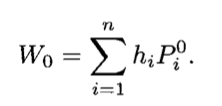
The first example is the shortfall probability in wealth management. Let us consider an investor who, in t=0, divides his assets among n different assets. The number of different assets is hi. Thus, his wealth in t=0 is given by the function:
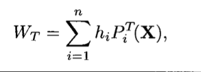
This portfolio is now held until time t = T. The price of the assets at time T depends on various risk factors such as inflation, the oil price or the general economic situation. Thus, the price at time T is determined by the following function, which takes these underlying factors into account:
Let X be a random variable. The final value of the portfolio is then given by this function:
Any number of observations can then be generated from this function using Monte Carlo. In this data set, it can then be evaluated how often a certain threshold was undercut.[8]
Monte Carlo Simulation
A good example of a Monte Carlo simulation is a simple autoregressive process. This is used in economics, for example, to describe the evolution of a quantity of interest over time. This could look like this, for example:
Here X0 is given and et is a random variable. This is random for each point in time (t = 1,2,3...). This noise term consists of a sequence of mutually independent and identically distributed normal random variables.[8]
In the first example, "Monte Carlo Sampling", the final value of X can be determined directly by the density function. In fact, no simulation is necessary. The PTi function is generated several times and then its properties are evaluated on the basis of the random experiments. In the second example, "Monte Carlo Simulation", a dynamic process is present. The value of Xt depends on its precursor Xt-1. This generates different paths. The dynamic model in Monte Carlo is usually described by a discrete-time, a continuous-time or a discrete event model. These examples suggest the definition that the term "sampling" is only used when no dynamics are generated over a time course, whereas this is exactly what happens with "simulations". In reality, however, these differences are often hardly to be made, since in both variants high-dimensional integrals of a function are often examined in order to make statements about a probability or expectation. [8]
Markov-Chain-Monte-Carlo Simulation
In reality, classical Monte Carlo simulation can sometimes reach its limits. This is especially the case when simulations are generated that have hundreds or thousands of unknown parameters. Therefore, Markov chain Monte Carlo simulations have been used since the 1950s. This was first done by Metropolis et at. (1953) to simulate a fluid in equilibrium with its gas state. They discovered that they did not need to simulate the exact dynamics, but only Markov chains that had the same equilibrium distribution. This is called the Metropolis algorithm. This was further developed in the 1970s into the Metropolis-Hastings algorithm, which is still highly relevant today. In a Markov chain, the variables follow a sequence of random elements X1,X2,...., where the conditional distribution of Xn+1 depends on Xn. Most Markov Chains in Monte Carlo simulations have a stationary transition probability if the conditional distribution of Xn +1 does not depend on Xn. In a simulation, for example, a sample of the generated variables is taken after a certain number of simulations and its properties are compared with the desired distribution. Depending on this, the next numbers are then simulated. With each further check, the distribution converges better and better with the desired one. Most Markov chains in simulation have an infinite state space, i.e. an infinitely large set of values of Xn. The theory of the Markov chain Monte Carlo simulation is the same as that of a conventional Monte Carlo simulation, but the statistical dependence of the random variables of the Markov chain changes the standard error.[9]
Characteristics Of A High Quality Monte Carlo Simulation
Sawilowsky defined in his paper "You Think You’ve Got Trivials?” in 2003 a number of characteristics that a high quaility Monte Carlo simulation should have. First, the pseudo number generator must have a number of properties, such as a long time series before individual numbers repeat. It must also pass tests for randomness. Furthermore, the number of repeated simulations must be sufficiently high. In addition, an appropriate sampling technique should be used. Moreover, the algorithm used must be valid for the model used. Finally, the model should actually simulate the described problem. If all these points are fulfilled, one can speak of a High Quality Monte Carlo Simulation.[10]
Problems with Monte Carlo Simulations
Critics accuse Monte Carlo simulation of being overused. Because it is often easy to use, scientists may prefer it to solving a problem analytically or experimentally. It should be noted that any simulation is only as good as its underlying model and input variables. However, this is not a general point of criticism, but is at most to be applied to the individual case. A general problem with Monte Carlo simulations, however, is computer time and memory, which are limited. This must be considered before creating a simulation to ensure that it can be run safely. Another problem is statistical and other errors. First of all, rounding errors can occur in the computer simulation due to a necessary limitation of decimal places. If these add up, this can lead to larger deviations depending on the simulation. Furthermore, a finite number of samples is always generated, which can lead to statistical errors that must be handled accordingly. [8]
Examples of Monte Carlo Simulations for Students
Throwing three dice
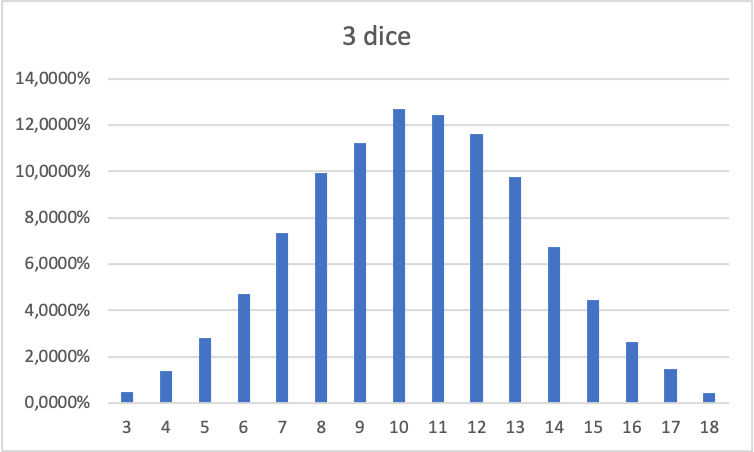
A first simple example of a Monte Carlo simulation is the simulation of cubes. This example can be used to explain how Monte Carlo works. Therefore, at this point it will also be explained how a simulation can be built in Excel. For example, if you have three dice, you can achieve a number between 3 and 18 with them. The different numbers have different probabilities. If there is only one combination for a 3 (1,1,1), there are already four possibilities for a 4 (1,1,2; 1,2,1; 2,1,1). In total, there are 6 x 6 x 6 = 216 different combinations of the dice. Theoretically, the different probability of each number between 3 and 18 can of course also be solved analytically, but it can also be easily done with a Monte Carlo simulation. To do this, let Excel throw 3 dices and then count the number of points. This process is repeated a few times to determine the corresponding probabilities. But let's proceed step by step.
The first step is to create three cubes. For this, the function =RANDBETWEEN(1;6) can be used in Excel. This function returns a random value between 1 and 6 with each update. The sum is then calculated in a fourth cell.
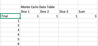
In the second step, a data table is created in which the results of the individual simulations are collected. To do this, first the header of the output table is transferred. The cells below are then equated with the cells of the original table. Then the rows below are numbered consecutively up to the desired simulation number. This can be done automatically in Excel by setting the desired final value under Home->Fill-> Series.
Excel can then run this simulation repeatedly in an automated manner. New random numbers are drawn each time. To do this, select the first row of the data table (with the transferred values) down to the last row in which results are to be saved. Then select Data -> What-if-analysis -> data table. For Column-input-cell select any free cell that Excel can use for calculation. Finally, you get the results of the individual simulations in the data table. For the number of points, for example, the following result is obtained after 10,000 simulations:
Calculation of π
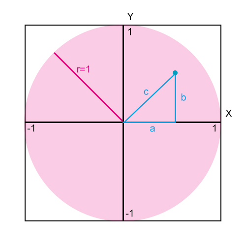
As already mentioned in the introduction to this article, the number Pi can also be calculated with a Monte Carlo simulation. To do this, create a coordinate system with the dimensions X€[-1;1] and Y€[-1,1]. From the center you create a circle with radius r=1. The probability that a random point lies on the circle is pi/4. In a Monte Carlo simulation, many random points are therefore generated on this coordinate system. Then pi=points in the circle/simulated points. The distance of the point from the center circle can be found using the Pythagoras theorem: d^2 = x^2 + y^2. If the distance is less than or equal to the radius of the circle. Then the point lies in the circle. In this example, the condition x^2 + y^2 <=1 results in the point being inside the circle. Since both variables are squared, it is sufficient to generate numbers in the range [0,1]. In Excel, this can be simulated by, for example, creating X and Y coordinates in cells A1 and B1 with the function =RAND(). Then check in C1 with the function =IF(POWER(A1,2 ) +POWER(B1,2)<=1;1;0) whether this point lies in the circle. This line is then copied again and again to create further points. With the function =SUM(C:C)/COUNT(C:C) you divide the hits on the circle by the number of simulations and get an approximation to the number Pi/4. To get Pi you have to multiply the result by 4.
File:Estimation of Pi example.xlsx
Evolution of Stock Prices
The last two examples already showed how Monte Carlo works in general and how it can be done in Excel. However, one important point is still missing for a complete Monte Carlo simulation, namely the time series. In the previous examples, an event was simulated repeatedly, but there was no relationship between the individual simulations. A good example of a complete simulation is the evolution of stock prices. It is assumed that the stock prices develop in a standard normal distribution.
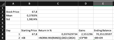
For example, the Moneta Money Bank share should be considered. This is, for example, at €67.80 at the moment. The aim is to find out how this share will develop over the next 30 trading days. To do this, we first have to look at the historical share prices. In the last 3 months, the share had an average daily return of 0.3783% with a standard deviation of 1.9824%.
For the first day, we enter the share's starting price of €67.80. Then simulate the price change for that day. Since this is standard normal distributed by assumption, this can be done in Excel with the function =NORM.INV(RAND();0.3783;1.9824). This random price change is multiplied by the starting price of the share to calculate the price gains/losses. The sum of this and the starting price of the share gives the final value of the share. This is then used as the starting value for the second trading day. The same procedure is followed for the next 29 days.
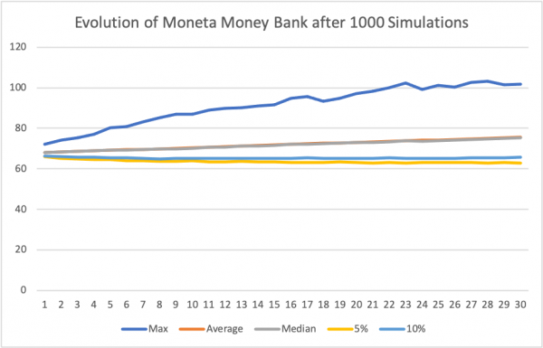
This gives a possible price development over 30 days. In order to make a statement about the development, this simulation must be repeated again and again. The easiest way to do this is to use the Data Tables function in Excel. Statistical evaluations can then be carried out on the basis of these different simulated paths. A possible development after 1000 simulations is shown in the figure. On the basis of this, it can be said that the stock price is on average 75.62€ and with 95% probability does not fall below a value of 62.87€. It must be said, however, that the number of simulations is quite low at 1000.
References
- ↑ IBM Cloud Education. What is Monte Carlo Simulation?[2020-01-24]. Available at: https://www.ibm.com/cloud/learn/monte-carlo-simulation#toc-what-is-mo-b7t4vgvP
- ↑ 2.0 2.1 2.2 2.3 2.4 Harrison, Robert L. Introduction To Monte Carlo Simulation. AIP Conf Proc. 2010 January 5; 1204: 17–21. doi:10.1063/1.3295638
- ↑ Richeson, David. A π-less Buffon's Needle Problem. Mathematics Magazine , Dec., 2006, Vol. 79, No. 5 (Dec., 2006), pp. 385-389. Available at: hhttps://www.jstor.org/stable/27642977
- ↑ Badger, Lee. Lazzarini's Lucky Approximation of π. Mathematics Magazine , Apr., 1994, Vol. 67, No. 2 (Apr., 1994), pp. 83-91. Available at: https://www.jstor.org/stable/2690682
- ↑ 5.0 5.1 Dizikies, Peter. Explained: Monte Carlo simulations: Mathematical technique lets scientists make estimates in a probabilistic world. MIT News. [17-05-2010] Available at: https://news.mit.edu/2010/exp-monte-carlo-0517
- ↑ Guillaume Chaslot, Sander Bakkes, Istvan Szita and Pieter Spronck. EMonte-Carlo Tree Search: A New Framework for Game AI. Proceedings of the Fourth Artificial Intelligence and Interactive Digital Entertainment Conference Available at: https://www.aaai.org/Papers/AIIDE/2008/AIIDE08-036.pdf
- ↑ Romeo, Giovanni. Chapter 14 - Essential Monte Carlo analysis, Elements of Numerical Mathematical Economics with Excel, Static and Dynamic Optimization,2020, Pages 763-795. Available at: https://doi.org/10.1016/B978-0-12-817648-1.00014-1
- ↑ 8.0 8.1 8.2 8.3 Brandimarte, Paolo. Handbook in Monte Carlo Simulation - Applications in Financial Engineering, Risk Management, and Economics. 2014. Published by John Wiley & Sons, Inc., Hoboken, New Jersey.
- ↑ Brook, Steve; Gelman, Andrew; Jones, Galin L.; Meng, Xiao-Li. Handbook of Markov Chain Monte Carlo. Chapman & Hall/CRC. 2012. USA
- ↑ Sawilowsky, Shlomo S. Invited Debate: Target Article You Think You’ve Got Trivials? Journal of Modern Applied Statistical Methods May, 2003, Vol. 2, No. 1, 218-225
