Difference between revisions of "Risk Simulation in Banking"
| Line 8: | Line 8: | ||
'''Approach:''' | '''Approach:''' | ||
| − | |||
| − | |||
| − | [[File:Regression Graph.png]] | + | [[File:Regression Graph.png|200px|thumb|left|]] |
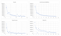
| + | Since there is no freely available data on the in-dept structure of the whole German banking market, the best approach is to simulate the environment based on samples. I | ||
| + | therefore picked the 18 largest in Germany operating banks together with several smaller ones and fitted a regression on the variables determining a banks bankruptcy. | ||
| + | Most interesting for stress-testing a bank is its balance sheet fundamentals. I chose to simulate the total Assets, Equity, Deposits and liquid Assets which I acquired by going | ||
| + | through their financial statements. With the fitted regression functions, I proceeded to project fictional banks to the point where total Assets on average equaled the total | ||
| + | Assets managed in the real market. | ||
| + | |||
| + | Total Assets = 3E+06x^(-1,389), | ||
| + | Equity = 154453x^(-1,43), | ||
| + | Deposits = 996993x^(-1,238), | ||
| + | Liquid Assets = 221117x^(-1,753) | ||
| − | |||
| − | |||
| − | |||
| − | |||
| − | |||
'''Method:''' | '''Method:''' | ||
I simulated geometric Brownian motions with a uniformly distributed multiplicator of m ϵ [0.8; 1.2] over 10 years for three of my four variables to represent the natural fluctuation of capital. The range for the multiplicator was arbitrarily set and could be specified further by a regression of the yearly change of the balance sheet information. Estimating the actual volatility of the yearly changes of the variables and introducing this information into the model would significantly increase the validity of the simulation. | I simulated geometric Brownian motions with a uniformly distributed multiplicator of m ϵ [0.8; 1.2] over 10 years for three of my four variables to represent the natural fluctuation of capital. The range for the multiplicator was arbitrarily set and could be specified further by a regression of the yearly change of the balance sheet information. Estimating the actual volatility of the yearly changes of the variables and introducing this information into the model would significantly increase the validity of the simulation. | ||
| + | |||
'''Detailed description:''' | '''Detailed description:''' | ||
| + | |||
There are basically two ways a bank can go bankrupt: | There are basically two ways a bank can go bankrupt: | ||
| Line 29: | Line 34: | ||
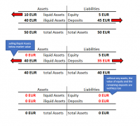
The first one is called a bank run. When customers lose trust in their bank, they might go and grab their deposits in order to save their money. Since the concept of fractional-reserve banking requires banks to only hold a share of it’s deposits as liquid cash, too many people collecting their deposits can dry up liquidity. The bank is forced to quickly sell their assets (even under their market value) to pay out their deposits. Once there is no more liquidity, the bank will need to file bankruptcy. | The first one is called a bank run. When customers lose trust in their bank, they might go and grab their deposits in order to save their money. Since the concept of fractional-reserve banking requires banks to only hold a share of it’s deposits as liquid cash, too many people collecting their deposits can dry up liquidity. The bank is forced to quickly sell their assets (even under their market value) to pay out their deposits. Once there is no more liquidity, the bank will need to file bankruptcy. | ||
| − | [[File:Bank run.png]] | + | [[File:Bank run.png|200px|thumb|left|]] I will simulate this by giving the bank run a possibility of 1/5000 to happen to a bank in year 0. If there is a bank run, a uniformly distributed portion between [0:x] of deposits will be deducted from the concerned banks liquid Assets. The ‘x’ can be specified on the ‘Overview’ sheet as ‘Deposit outflow (bank runs, upper limit)’ to vary the percentage of deposits withdrawn. |
| − | |||
| − | I will simulate this by giving the bank run a possibility of 1/5000 to happen to a bank in year 0. If there is a bank run, a uniformly distributed portion between [0:x] of deposits will be deducted from the concerned banks liquid Assets. The ‘x’ can be specified on the ‘Overview’ sheet as ‘Deposit outflow (bank runs, upper limit)’ to vary the percentage of deposits withdrawn. | ||
If the liquidity is not sufficient to cover the extent of the bank run, the bank goes bankrupt. | If the liquidity is not sufficient to cover the extent of the bank run, the bank goes bankrupt. | ||
Every bankrupt bank increases the probability of another bank getting a bank run by 1% since customers do not trust their deposits safety anymore. This is, to simulate the possibility of a Snowball effect where healthy banks get bank runs because of panics in the overall sector. | Every bankrupt bank increases the probability of another bank getting a bank run by 1% since customers do not trust their deposits safety anymore. This is, to simulate the possibility of a Snowball effect where healthy banks get bank runs because of panics in the overall sector. | ||
One can vary the initial amount of liquidity in year 0 by changing the ‘Liquidity multiplicator’ on the ‘Overview’ sheet to experiment with the effect, different liquidity levels do have on the bankruptcy chance. | One can vary the initial amount of liquidity in year 0 by changing the ‘Liquidity multiplicator’ on the ‘Overview’ sheet to experiment with the effect, different liquidity levels do have on the bankruptcy chance. | ||
| + | |||
| + | |||
| + | |||
| + | |||
| + | |||
'''Asset Price Shock:''' | '''Asset Price Shock:''' | ||
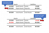
The other main way for a bank to become bust is due to shocks to asset prices. If prices of the financial assets of the bank deflate while the deposits values are contractually fixed, the equity needs to decrease in order to balance out the financial statement. Once the asset prices dragged the equity to zero, bankruptcy is almost inevitable. | The other main way for a bank to become bust is due to shocks to asset prices. If prices of the financial assets of the bank deflate while the deposits values are contractually fixed, the equity needs to decrease in order to balance out the financial statement. Once the asset prices dragged the equity to zero, bankruptcy is almost inevitable. | ||
| − | [[File:Asset price shock.png]] | + | [[File:Asset price shock.png|200px|thumb|left|]] Same as bank runs, asset depreciation rarely concerns just one bank. Usually banks invest in a similar asset basket and market selloffs hit all of them in a comparable way. Therefore, the same chances of 1/5000 at t=0, with an increase of 1% for every bankrupt bank is put in place here too. |
| − | |||
| − | Same as bank runs, asset depreciation rarely concerns just one bank. Usually banks invest in a similar asset basket and market selloffs hit all of them in a comparable way. Therefore, the same chances of 1/5000 at t=0, with an increase of 1% for every bankrupt bank is put in place here too. | ||
The real-world solution for fluctuating asset prices in banking is hedging. If the introduction of hedging is done right, the total asset position can be kept relatively stable since decreases in some assets are balanced out by increases in the value of the hedging instruments. | The real-world solution for fluctuating asset prices in banking is hedging. If the introduction of hedging is done right, the total asset position can be kept relatively stable since decreases in some assets are balanced out by increases in the value of the hedging instruments. | ||
The way I modeled this is by introducing variable upper and lower limits for the asset price change in one given year. They too, can be found on the ‘Overview’ sheet. | The way I modeled this is by introducing variable upper and lower limits for the asset price change in one given year. They too, can be found on the ‘Overview’ sheet. | ||
Another method used for reducing the risk of asset price fluctuations is the increase of Equity. Similar to what I did with the liquidity, one can change the initial level of Equity on the ‘Overview’ sheet by changing the ‘Equity multiplicator’. | Another method used for reducing the risk of asset price fluctuations is the increase of Equity. Similar to what I did with the liquidity, one can change the initial level of Equity on the ‘Overview’ sheet by changing the ‘Equity multiplicator’. | ||
| + | |||
| + | |||
| + | |||
'''Bailouts:''' | '''Bailouts:''' | ||
Due to the risk of snowball effects, Governments oftentimes intervene when they see the danger of a financial institutions going insolvent. Therefore, I modeled a bailout option where one can put the maximum number of bailouts per year. | Due to the risk of snowball effects, Governments oftentimes intervene when they see the danger of a financial institutions going insolvent. Therefore, I modeled a bailout option where one can put the maximum number of bailouts per year. | ||
| + | |||
| + | |||
'''Results:''' | '''Results:''' | ||
| + | |||
'''Test 1.: increasing bailout willingness''' | '''Test 1.: increasing bailout willingness''' | ||
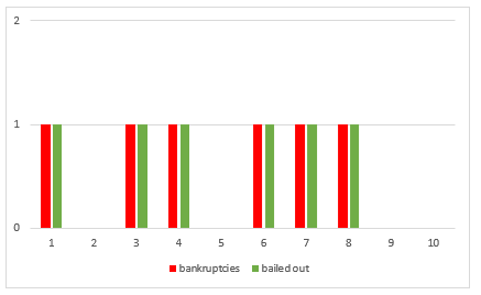
The first simulation run was done using a Liquidity-, and Equity multiplicator of 1, a uniformly distributed interval of ϵ [0; 0.5] for the deposit outflows and an interval of ϵ [0.8; 1.2] for the Brownian motion. The maximum number of bailouts per year was initially set to 0. | The first simulation run was done using a Liquidity-, and Equity multiplicator of 1, a uniformly distributed interval of ϵ [0; 0.5] for the deposit outflows and an interval of ϵ [0.8; 1.2] for the Brownian motion. The maximum number of bailouts per year was initially set to 0. | ||
Revision as of 15:07, 20 January 2021
Risk Simulation in Banking
Problem: Modern Banking is a highly volatile business with interdependencies not only to other banks, but to the economy as a whole, too. It is therefore that most of the economic crisis of the past century had been accelerated or caused entirely by the financial sector. Because of the interdependencies and to avoid snowball effects when one financial institute tumbles, regulators began to introduce different sorts of safety mechanisms. My goal is, to simulate the German banking market and deduct default probabilities with varying extends of banking regulation in place.
Approach:
Since there is no freely available data on the in-dept structure of the whole German banking market, the best approach is to simulate the environment based on samples. I therefore picked the 18 largest in Germany operating banks together with several smaller ones and fitted a regression on the variables determining a banks bankruptcy. Most interesting for stress-testing a bank is its balance sheet fundamentals. I chose to simulate the total Assets, Equity, Deposits and liquid Assets which I acquired by going through their financial statements. With the fitted regression functions, I proceeded to project fictional banks to the point where total Assets on average equaled the total Assets managed in the real market.
Total Assets = 3E+06x^(-1,389), Equity = 154453x^(-1,43), Deposits = 996993x^(-1,238), Liquid Assets = 221117x^(-1,753)
Method: I simulated geometric Brownian motions with a uniformly distributed multiplicator of m ϵ [0.8; 1.2] over 10 years for three of my four variables to represent the natural fluctuation of capital. The range for the multiplicator was arbitrarily set and could be specified further by a regression of the yearly change of the balance sheet information. Estimating the actual volatility of the yearly changes of the variables and introducing this information into the model would significantly increase the validity of the simulation.
Detailed description:
There are basically two ways a bank can go bankrupt:
Bank runs: The first one is called a bank run. When customers lose trust in their bank, they might go and grab their deposits in order to save their money. Since the concept of fractional-reserve banking requires banks to only hold a share of it’s deposits as liquid cash, too many people collecting their deposits can dry up liquidity. The bank is forced to quickly sell their assets (even under their market value) to pay out their deposits. Once there is no more liquidity, the bank will need to file bankruptcy.
I will simulate this by giving the bank run a possibility of 1/5000 to happen to a bank in year 0. If there is a bank run, a uniformly distributed portion between [0:x] of deposits will be deducted from the concerned banks liquid Assets. The ‘x’ can be specified on the ‘Overview’ sheet as ‘Deposit outflow (bank runs, upper limit)’ to vary the percentage of deposits withdrawn.
If the liquidity is not sufficient to cover the extent of the bank run, the bank goes bankrupt. Every bankrupt bank increases the probability of another bank getting a bank run by 1% since customers do not trust their deposits safety anymore. This is, to simulate the possibility of a Snowball effect where healthy banks get bank runs because of panics in the overall sector. One can vary the initial amount of liquidity in year 0 by changing the ‘Liquidity multiplicator’ on the ‘Overview’ sheet to experiment with the effect, different liquidity levels do have on the bankruptcy chance.
Asset Price Shock:
The other main way for a bank to become bust is due to shocks to asset prices. If prices of the financial assets of the bank deflate while the deposits values are contractually fixed, the equity needs to decrease in order to balance out the financial statement. Once the asset prices dragged the equity to zero, bankruptcy is almost inevitable.
Same as bank runs, asset depreciation rarely concerns just one bank. Usually banks invest in a similar asset basket and market selloffs hit all of them in a comparable way. Therefore, the same chances of 1/5000 at t=0, with an increase of 1% for every bankrupt bank is put in place here too.
The real-world solution for fluctuating asset prices in banking is hedging. If the introduction of hedging is done right, the total asset position can be kept relatively stable since decreases in some assets are balanced out by increases in the value of the hedging instruments. The way I modeled this is by introducing variable upper and lower limits for the asset price change in one given year. They too, can be found on the ‘Overview’ sheet. Another method used for reducing the risk of asset price fluctuations is the increase of Equity. Similar to what I did with the liquidity, one can change the initial level of Equity on the ‘Overview’ sheet by changing the ‘Equity multiplicator’.
Bailouts:
Due to the risk of snowball effects, Governments oftentimes intervene when they see the danger of a financial institutions going insolvent. Therefore, I modeled a bailout option where one can put the maximum number of bailouts per year.
Results:
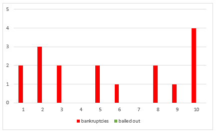
Test 1.: increasing bailout willingness The first simulation run was done using a Liquidity-, and Equity multiplicator of 1, a uniformly distributed interval of ϵ [0; 0.5] for the deposit outflows and an interval of ϵ [0.8; 1.2] for the Brownian motion. The maximum number of bailouts per year was initially set to 0. Each setting, I run 50 times, with one run simulating 10 years, giving a sample size of 500 bank years per setting. After that, the number of possible bailouts was increased by 2.
The willingness to bail out struggling financial institutions does have a significant influence both on the expected number of defaults same as on the standard deviation. With a maximum of 4 bailouts, the probability for a default nearly halves from 1,98 to 1 per 10-year interval, while standard deviation decreased from 3,09 to 1,60.
Test 2.: Increased Liquidity Second, I simulated the effect an increase in liquidity would have on the default probability.
Not surprisingly, an increased liquidity reduced the average default probability and its standard deviation. However, the results have not been as robust as in the case of the bailouts. This might be due to limitations in the model: While I assumed that in the case of a bank run a uniformly distributed amount of ϵ [0; 0.5] of deposits gets liquidated immediately, most of the deposits a bank has are contractually fixed to be paid out only after a cancelation period of anywhere between 1 week to 3 months, giving the banks enough time to organize a adequate amount of cash. Also, in the European Union, there is a deposit insurance, guaranteeing 100.000€ per customer per institution in case of insolvencies, which additionally reduces the chances of bank runs and liquidity squeezes. Therefore, financial institutions require fewer liquid assets than my model would suggest. Which led to an overestimate of the default probability caused by a seemingly lack of liquidity.
Test 3: Increasing Equity
I tested which influence increasing Equity would have on the default probability.
Same as in the case of Liquidity, the results show a slight decrease in default probability for increasing Equity. However, for an increase in Equity by 100%, one would expect a more extreme decrease in the average number of bankruptcies.
Test 4: Increasing Equity, Liquidity and the willingness to bail out
In the last testing sequence, I tested the impact of all three variables together.
Again, one is able to observe significant reductions in the average default probability. After the first three tests it seems likely that the effect is dominated by the willingness to bail out, which appears to be the single biggest influencer when it comes to reducing the number of bankruptcies in the model.
Conclusion: Within the limitations of the model, bailing out struggling institutions seems to be the most promising way of government intervention when it comes to reducing the likeliness of a financial crisis. An increase in the maximum allowed number of bail outs from 0 to 4 reduced the average bankruptcy amount in 10 years by almost 50%. Note that an increased willingness to bail out does not have a direct effect on the base probability for bankruptcies. However, bailed out institutions are not able to kick off a chain reaction of bankruptcies and therefore reduce the overall probability of default.
When it comes to Equity and Liquidity increases, the results are not that clear. In theory, both should reduce the default probability greatly while the model only showed small effects. One reason for this is of course that real institutions are not static. When they realize the market environment is changing and becoming more risky, it is good practice to stock up on Liquidity. An Effect which is not visible in the year-to-year balance sheet information and therefore did not find its way into the model. Also, as mentioned before, the Liabilities in form of customer deposits usually need to be canceled first before they can be accessed by the depositor. A more sophisticated model for bank runs should include a concept like Duration to model the in- and outflow of liquidity in a more realistic, day-to-day way. It is for these two reasons that the Liquidity and Equity Quotas I observed in the balance sheet information seem to be too low for effectively reducing default risks in my model. However, thinking about the incentive problems that come with bail outs it would not be advisable to only rely on the tool of government money for avoiding a financial crisis.
