Difference between revisions of "Retirement Planning"
(→Conclusion) |
(→Input Variables) |
||
| (3 intermediate revisions by the same user not shown) | |||
| Line 117: | Line 117: | ||
U.S. government bonds have historically never defaulted, so there is no default risk. Moreover, there has never been a Black Swan year. It should be noted that the standard normal distribution can also lead to negative interest rates. Although this has not occurred historically with U.S. government bonds, it is theoretically conceivable (see German government bonds). At a time when discussions about negative interest rates for private investors are being held again and again, this assumption seems realistic. | U.S. government bonds have historically never defaulted, so there is no default risk. Moreover, there has never been a Black Swan year. It should be noted that the standard normal distribution can also lead to negative interest rates. Although this has not occurred historically with U.S. government bonds, it is theoretically conceivable (see German government bonds). At a time when discussions about negative interest rates for private investors are being held again and again, this assumption seems realistic. | ||
| + | |||
| + | For the investment in the 5 preceding years, an equal distribution of 20% each was chosen. In addition, the real YTMs (Yield to Maturity) were chosen. These were: | ||
| + | |||
| + | 2016: 1,3194% | ||
| + | |||
| + | 2017: 1,9161% | ||
| + | |||
| + | 2018: 2,7328% | ||
| + | |||
| + | 2019: 1,8985% | ||
| + | |||
| + | 2020: 0,4506% | ||
== Results == | == Results == | ||
| Line 177: | Line 189: | ||
== Excel File == | == Excel File == | ||
| + | |||
| + | [[File:Retirement Simulation.xlsx]] | ||
Latest revision as of 22:03, 19 January 2021
Contents
Problem Definition
In retirement planning, there are different investment options that are associated with different risks. Therefore, this simulation is intended to help compare different investment options and evaluate their risk. For this purpose, it is assumed that a fixed amount is already invested in one of the options and that a fixed amount will be invested over the next 30 years. Two different options are compared, an investment in a chosen stock portfolio or an investment in bonds. To make the model more realistic, it is assumed that the stock markets are repeatedly shaken by black swan events. Black swan events are, for example, financial crises that occur irregularly and without warning. In addition, inflation is simulated over the next 30 years and the result are adjusted for it.
Method
The chosen simulation method is a Monte Carlo simulation in Excel.
Model
Inflation
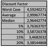
Inflation is assumed to be normally distributed. For the simulation, both a mean value and the standard deviation must be determined. Then the discount factors for each simulation are calculated. The result of the two investment options is in the end adjusted by a selection from these discount factors. The worst case scenario, the mean, the median and the 5%, 10%, 15%, 20% percentile (5% percentile is the value that is not exceeded with 95% certainty) were chosen. Inflation is simulated 1000 times.
Stock Portfolio
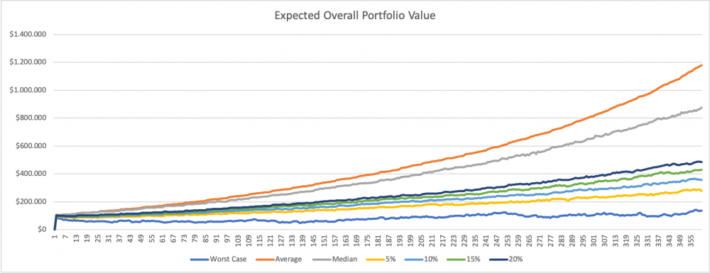
A fixed amount is already paid in at the beginning of the simulation and a fixed amount is invested each year in January. The results from the stock portfolio are standard normally distributed and are calculated on a monthly basis. However, a distinction must be made between two scenarios. A mean and a standard deviation are required for months in which a black swan event occurs and for months in which no black swan event occurs. In addition, a probability must be given for the occurrence of a Black Swan month. The simulation then randomly determines whether a month is a Black Swan month or not. The results of the Monte Carlo simulation record how many Black Swan months occurred in a simulation. This makes it possible to examine the results afterwards for the number of Black Swan months.The Stock portfolio is simulated 1000 times.
The stock portfolio consists of a mixture of an investment in the S&P 500 and a portfolio of 4 DAX stocks. The optimal weights for both portfolios were determined using a Monte Carlo simulation. Random weights are assigned to the individual stocks and the respective expected return and variance are calculated from the combination. Since the portfolio is a retirement plan, the weights were chosen in such a way that the portfolio has a minimum risk (minimum variance / standard deviation). 1000 different weights are choosen for both optimisations.
Bond Investment
The second investment option is an investment in bonds. For this, 5-year government bonds were chosen because they are practically risk-free and the money is invested for a manageable period of time and is therefore quite liquid. These government bonds pay interests annually. The annual interest rate of each year is standard normal distributed and a mean value and a standard deviation are required. An annual interest gain is thus generated each year from the government bonds from the last 5 years. This accrued interests are reinvested at the beginning of each year. In addition, the invested amount is paid back after 5 years and reinvested in government bonds. To make the value of these investments comparable with a stock portfolio, the total amount invested is considered. Since the majority of the investment is only made every 5 years when the full amount is invested at the beginning of the simulation, it is assumed that the strategy has already been implemented in the last 5 years. This ensures an even distribution over the years. The Bond portfolio is simulated 1000 times.
General Comments
To make this simulation a general-purpose tool, all assumptions for the simulation can be set and changed in the worksheet "Setting" (green tab). My selected values are in column D for orientation, but the simulations work with the values from column C.
First, the weights in the DAX portfolio and the weights of the distribution between the DAX portfolio and the S&P 500 can be changed. If these weights are changed, an estimate of the mean and standard deviation in regular months and in Black Swan months is obtained in cells D29:D40. The probability of a Black Swan month is also given. A black swan month is defined as a month in which the return falls below the mean by at least 2.5 times the standard deviation. These values are calculated on the basis of a hypothetical portfolio with the selected weights between 6.1998 and 1.2021. The mean and standard deviation are then calculated separately for months with and without Black Swan. Theoretically, however, one can also ignore the selected shares and provide one's own data on the distribution. The selected weights only have an influence on the suggestions in column D. In addition, the assumptions about the previous bond investment from 2016-2020 can also be set.
If the selected settings are changed, the simulations (blue tabs) must be recalculated. The automatic calculation of data tables is switched off due to the size of the file. Data Tables can be recalculated under Formulas -> Calculate Now. However, this can lead to problems with low performance computers. Then the 3 simulations (blue tabs) can be calculated individually by switching to the worksheet and pressing Formulas -> Calculate Sheet.
Input Variables
Black Swan Definition
A black swan month is defined as a month in which the return falls below the mean by at least 2.5 times the standard deviation.
Starting Balance
A starting balance of $100,000 was chosen. Since the simulation works exclusively with percentages, the selected currency only has an influence on inflation.
Yearly Contribution
A yearly contribution of $5,000 was chosen.
Inflation
US dollars were chosen as the currency. This has the simple reason that there is a comparably long history here. The data for this was taken from the Worldbank.
Historical mean: 3.7208%
Historical Standard Deviation: 2.7783%
Stock Portfolio
All Stock Data was obtained from Yahoo Finance.
Initially, 4 shares were selected for the DAX portfolio. These 4 shares are: Adidas, Deutsche Bank, Siemens and Volkswagen.
With the help of a Monte Carlo simulation and a random distribution of weights on the 4 stocks, the portfolio with a minimum risk was determined (minimum standard deviation). For this purpose, the covariance was used on the basis of historical data.
The weights in this portfolio are:
Adidas: 44.4905%
Deutsche Bank: 9.7501%
Siemens: 20.7922%
Volkswagen: 24.9672%
Afterwards, a Monte Carlo simulation was used to find the best allocation between this DAX portfolio and an investment in the S&P 500. Historical data and the covariance were used for this.
The weights in this portfolio are:
DAX portfolio: 7.4357%
S&P 500: 92.5643%
With these weights, a hypothetical portfolio was created between 6/1998 and 1/2021. This hypothetical portfolio considers 271 months, 5 of which fall under the chosen Black Swan definition.
This results in:
Monthly Mean Return without Black Swan Months: 0.7961%
Monthly Std without Black Swan Months: 4.0648%
Probability of a black swan month: 1,8450%
Monthly Mean Return of Black Swan Months: -13.1630%
Monthly Std of Black Swan Months: 2.4150%
This are the settings that I chose for my simulation. The combination of different stocks leads to the fact that data can only be used in the period in which it is available for all 5 stocks. Therefore, a simulation with a pure investment in S&P 500 stocks is also interesting. Here data is available for 1117 months (18 Black Swan Months). The values for such a simulation can be found in the Excel file in the tab "S&P 500 Data" in column T. Also for pure investments in all other stocks the data is available in the corresponding Data Worksheet (red tabs). The new values can be easily entered in the "Settings" worksheet.
Bond Investment
For this bond data, 5-year U.S. government bonds were chosen since the data go back to 1962. Based on historical interest rates, the following values were determined:
Mean yearly YTM: 5.6864%
Std of yearly YTM: 3.1610%
U.S. government bonds have historically never defaulted, so there is no default risk. Moreover, there has never been a Black Swan year. It should be noted that the standard normal distribution can also lead to negative interest rates. Although this has not occurred historically with U.S. government bonds, it is theoretically conceivable (see German government bonds). At a time when discussions about negative interest rates for private investors are being held again and again, this assumption seems realistic.
For the investment in the 5 preceding years, an equal distribution of 20% each was chosen. In addition, the real YTMs (Yield to Maturity) were chosen. These were:
2016: 1,3194%
2017: 1,9161%
2018: 2,7328%
2019: 1,8985%
2020: 0,4506%
Results
Inflation
The simulation of inflation leads to the following discount factors:
Stock Portfolio
The expected evolution of the portfolio value is shown in this graphic:
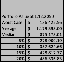
The following table contains the corresponding final values:
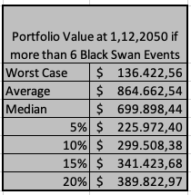
In addition, the Excel file can be used to exclude simulations that contain a certain number of Black Swan events. For example, if you exclude all simulations that contain less than 7 Black Swan months, you will get the following results:
Finally, the results are adjusted for the results of the inflation simulation:
Bond Investment
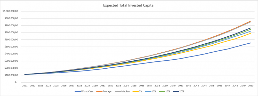
The expected evolution of the total invested capital is shown in this graphic:
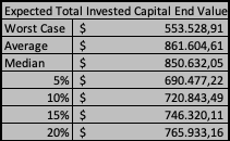
The following table contains the corresponding final values:
Finally, the results are adjusted for the results of the inflation simulation:
Conclusion
In conclusion, it can be said that an investment in the selected stock portfolio is significantly riskier. Although it holds the possibility of high profits, on the other hand, it also holds harsh losses. In particular, the stock portfolio is strongly dependent on how many Black Swan months occur.
The investment in government bonds, on the other hand, is much safer, but also has lower chances of extremely high profits.
In the end, it is up to each individual to decide which portfolio to invest in. However, since it is a pension plan and the risk profile of both investments is very different, I think that most people choose to invest in government bonds.
